Drug Discovery Trends In and From the Literature

I came across a recent paper by Agarwal and Searls which describes a detailed bibliometric analysis of the scientific literature to identify and characterize specific research topics that appear to be drivers for drug discovery – i.e., research areas/topics in life sciences that exhibit significant activity and thus might be fruitful for drug discovery efforts. The analysis is based on PubMed abstracts, citation data and patents and addresses research topics ranging from very broad WHO disease categories (such as respiratory infectins and skin diseases) to more specific topics via MeSH headings and down to the level of indivudal genes and pathways. The details of the methodology are described in a separate paper, but this one provides some very interesting analyses and visualizations of drug discovery trends.

The authors start out by defining the idea of “push” and “pull”:

Unmet medical need and commercial potential, which are considered the traditional drivers of drug discovery, may be seen as providing ‘pull’ for pharmaceutical discovery efforts. Yet, if a disease area offers no ‘push’ in the form of new scientific opportunities, no amount of pull will lead to new drugs — at least not mechanistically novel ones …

The authors then describe how they characterized “push” and “pull”. The key premise of the paper is that publications rates are an overall measure of activity and when categorized by topic (disease area, target, pathway etc), represent the activity in that area. Of course, there are many factors that characterize why certain therapeutic or target areas receive more interest than others and the authors clearly state that even their concepts of “push” and “pull” likely overlap and thus are not independent.

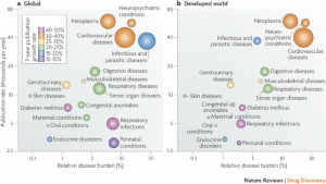
For now I’ll just highlight some of their analysis from the “pull” category. For example, using therapeutic areas from a WHO list (that characterized disease burden) and PubMed searches to count the number of papers in a given area, they generated the plot below. The focus on global disease burden and developed world disease burden was based on the assumption that the former measures general medical need and the latter measures commercial interest.

Figure 2 from Agarwal and Searls

Figure 2 from Agarwal and Searls

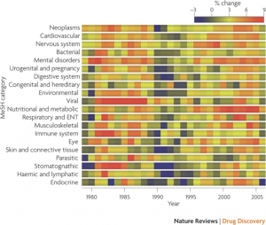
Another interesting summary was the rate of change of publication in a given area (this time defined by MeSH heading). This analysis used a 3 year window over a 30 year period and highlighted some interesting short term trends – such as the spurt in publications for viral research around the early 80’s which likely corresponded to discovery of retroviral involvement in human disease and then later by the AIDS epidemic. The data is summarized in the figure below, where red corresponds to a spurt in activity and blue to a stagnation in publication activity.

Figure 4 from Agarwal and Searls

They also report analyses that focus on high impact papers, based on a few of the top tier journals (as identified by impact factor) – while their justification is reasonable, it does have downsides which the authors highlight. Their last analysis focuses on specific diseases (based on MeSH disease subcategories) and individual protein targets, comparing the rate of publications in the short term (2 year windows) versus medium term (5 year windows). The idea is that this allows one to identify areas (or targets etc) that exhibit consistent growth (or interest), accelerating and decelerating growth . The resultant plots are quite interesting – though I wonder about the noise involved when going to something as specific as individual targets (identified by looking for gene symbols and synonyms).

While bibliometric analysis is a high level approach the authors make a compelling case that the technique can identify and summarize the drug discovery research landscape. The authors do a great job in rationalizing much of their results. Of course, the analyses are not prospective (i.e., which area should we pour money into next?). I think one of the key features of the work is that it quantitatively characterizes research output and is able to link this to various other efforts (specific funding programs, policy etc) – with the caveat that there are many confounding factors and causal effects.
A Custom Palette for Heatmaps

Heatmaps are a common way to visualize matrices and R provides a variety of methods to generate these diagrams. One of the key features of a heatmap is the color scheme employed. By default the image method uses heat.colors which ranges from red (lowest values) to white (highest values). Other palettes include rainbow and topographical. However, I needed to replicate a color scheme used in a previous publication – dark red for low values and white for high values, passing through shades of pink. While RColorBrewer is an extremely useful package for generating sensible and informative color schemes it didn’t help me out here – the red palette was limited to 9 colors, whereas I needed a larger range. There’s also the colorschemes method from the ClassDiscovery package, but I haven’t checked that out.

So, I ended up making my own color scheme, realizing that shades of pink are a constant red, coupled with increasing amounts of blue and green (in the RGB scheme). Thus generating a matrix of R, G and B values, with a constant red value and increasing blue and green values and then converting the rows to hex colors (via rgb, gives me the required colors.

1
2
3
4
rgbs <- cbind(255,
                     seq(32,255, length=256),
                     seq(32,255, length=256)) / 255
cols <- rgb(rgbs[,1], rgbs[,2], rgbs[,3])

and an example of the color scheme

1
2
image(matrix(1:256, nrow=64, byrow=TRUE),
           col=cols)

resulting in

Correlating Continuous and Categorical Variables

At work, a colleague gave an interesting presentation on characterizing associations between continuous and categorical variables. I expect that I will be facing this issue in some upcoming work so was doing a little reading and made some notes for myself.

Given a continuous variable Y and a categorical variable G, is the distribution of Y independent of the levels of G? One can address this using parametric or non-parametric methods. Due to the superior power of parametric methods we start by considering them and only if we completely fail to satisfy the distributional assumptions of such methods, do we move to the non-parametric methods.

A simple approach is to convert G to an indicator variable matrix, such that each level of G becomes a binary vector, and then use this matrix and Y to fit a linear model. One can then perform an ANOVA on the fit to check whether Y is independent of the groups. This approach assumes that Y is normally distributed, and that variances are equal amongst the groups.

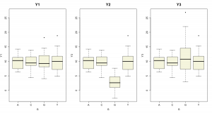
A simple example in R is as follows. We first create a dataset in which there is no difference in the mean or variance across the groups, one in which the means differ and one in which the variances differ

1
2
3
4
5
6
7
8
9
10
11
G <- factor(sample(c('A','T','C','G'),
                     100,
                     TRUE,
                     c(0.2,0.2,0.2,0.2)))
Y1 <- rnorm(100, mean=10, sd=3)

Y2 <- Y1
Y2[which(G=='G')] <- sample(rnorm(length(which(G=='G')),mean=4,sd=3))

Y3 <- Y1
Y3[which(G=='G')] <- sample(rnorm(length(which(G=='G')),mean=10,sd=6))

A summary of the Y’s grouped by G are given below.

We now run the ANOVA, using the first dataset.

1
2
fit <- lm(Y1 ~ G, data=data.frame(Y1,G))
anova(fit)

Running this gives us

1
2
3
4
5
Analysis of Variance Table
         Response: Y1
          Df Sum Sq Mean Sq F value Pr(>F)
G          3   0.74    0.25  0.0304 0.9928
Residuals 96 777.19    8.10

If we consider the 0.05 significance level, we would not reject the null hpothesis that Y is independent of G. If we now rerun the ANOVA using the second dataset

1
2
fit <- lm(Y2 ~ G, data=data.frame(Y2,G))
anova(fit)

we get

1
2
3
4
5
Analysis of Variance Table
         Response: Y2
          Df  Sum Sq Mean Sq F value    Pr(>F)
G          3 1131.65  377.22  49.321 &lt; 2.2e-16 ***
Residuals 96  734.22    7.65

which suggests that we reject the null hypothesis and accept the alternative that there is the Y’s are not independent of the groups (which is true by design).

Furthermore, it really only indicates whether there is a dependence between the groups and the means of the group members – it doesn’t tell us anything about lack of independence in terms of scale parameters. This is not surprising since the linear model is defined to have a constant variance. Thus, if we want to investigate dependence of the variance on groups, we should look at distributions of residuals or other approaches to identifying heteroscedacity (such as Levenes test).

In case we cannot satisfy the assumptions (even after investigating possible transformations of the data) required for ANOVA, we can move to parametric methods, which are easy to run, but have a lower power. For this problem, the Kruskal-Wallis test and the Fligner-Killeen test come in handy. These methods are in the base stats package but also come with the coin package which is handy for running a variety of independence tests.

The Kruskal-Wallis test makes no assumptions about normality, but does assume that the distributions amongst the levels of G are of the same shape and have the same variance (and so, the differences are due to differences in the means). The Fligner-Killeen test also avoids the normality assumption bu in this case, has the null hypothesis that the variances in the groups are the same. Thus ideally, we’d run the Kruskal-Wallis first and if we could not reject the null hypothesis we then investigate whether there is a difference in the variances across the groups by the Fligner-Killeen tests.

Some examples highlight the analysis. First, we consider the dataset that is independent of the groups (Y1):

1
2
3
4
5
6
> kruskal_test(Y1 ~ G, data=data.frame(Y1,G))

    Asymptotic Kruskal-Wallis Test

data:  Y1 by G (A, C, G, T)
chi-squared = 0.0628, df = 3, p-value = 0.9959

which indicates that we fail to reject the null hypothesis that the distribution of Y1 is independent of the levels of G. We then consider the dataset where the means are dependent on the groups

1
2
3
4
5
6
> kruskal_test(Y2 ~ G, data=data.frame(Y2,G))

    Asymptotic Kruskal-Wallis Test

data:  Y2 by G (A, C, G, T)
chi-squared = 57.3197, df = 3, p-value = 2.196e-12

which indicates the we can reject the null hypothesis. However, note that for Y3, where the means are independent of the groups but the variance differ, the Kruskal-Wallis test is not useful:

1
2
3
4
5
6
> kruskal_test(Y3 ~ G, data=data.frame(Y3,G))

    Asymptotic Kruskal-Wallis Test

data:  Y3 by G (A, C, G, T)
chi-squared = 1.5399, df = 3, p-value = 0.673

On the other hand, if we run the Fligner-Killeen test on these three datasets, we correctly identify Y3 as having its variance dependent on G

1
2
3
4
5
6
7
8
9
10
11
12
13
14
15
16
17
18
19
20
> fligner_test(Y1 ~ G, data=data.frame(Y1,G))

    Asymptotic Fligner-Killeen Test

data:  Y1 by G (A, C, G, T)
chi-squared = 2.9914, df = 3, p-value = 0.3929

> fligner_test(Y2 ~ G, data=data.frame(Y2,G))

    Asymptotic Fligner-Killeen Test

data:  Y2 by G (A, C, G, T)
chi-squared = 2.8202, df = 3, p-value = 0.4202

> fligner_test(Y3 ~ G, data=data.frame(Y3,G))

    Asymptotic Fligner-Killeen Test

data:  Y3 by G (A, C, G, T)
chi-squared = 15.3493, df = 3, p-value = 0.001541

Oracle Notes

Some handy settings when running a query from the command line via sqlplus

set echo off
set heading on
set linesize 1024
set pagesize 0
set tab on
set trims on
set wrap off
-- might want to set column formats here
-- e.g.: column foo format A10
spool stats -- dump results to stats.lst
-- SQL query here

spool off
exit

Switching from the Chair to the Bed

The Fall ACS meeting, held in Washington DC, is over and I can get back to breathing. The CINF program at the meeting was excellent (but I’m biased) with a variety of symposia. Notable amongst them was the Herman Skolnik symposium, honoring this years Herman Skolnik awardee, Yvonne Martin. Of all the talks, two that caught my eye. Jonathan Goodmans’ talk showed the first case of an InChI key collision, which appears to have been confirmed by ChemSpider and Symyx. The second talk was by Anthony Nicholls of OpenEye at the Herman Skolnik symposium. He discussed the issue of ‘hyperparametric modeling’, i.e., the fact that many types of models ranging from QSAR to molecular dynamics and ab initio methods are over paarmetrized. While this problem is very obvious in QSAR modeling (hence feature selection), the implicit parametrization in things like force fields, ab initio methods is not always obvious. He also discussed issues with model validation techniques such as cross-validation and y-scrambling and suggested techniques that might be better to assess a model. In essence he suggests that we will be more rigorous about model quality when we start assesing the “risk” of a bad model, rather than just how well the model fits the data (which can obviously be misleading). While these ideas are not brand new, the examples and the presentation were eye opening. The last talk in General Papers on Thursday was also quite interesting – B.-Y. Jin spoke about topological rules defining the structures of various nanotube and fullerene structures and how he had been constructing them as bead models. Examples of them can be found on his blog .

I was also involved in organizing a symposium on scripting and programming with COMP. We initially feared that the topic might be too geeky, but we were pleasntly surprised by the size of the audience. We had speakers talking about their favorite languages and how they do modeling and cheminformatics using them. I spoke about R and rcdk – which turned out to be so hot that we were interrupted by a fire alarm (three times!)

On the social events side of things, it was good to meet up with old friends and make new ones. CINF hosted a number of receptions, all excellent. A dinner for CINF functionaries was held at Zaytinya – a Mediterranean tapas restaurant. All I can say is: mindblowing! I had never realized that shrimp and dill could be such a killer combination. The Blue Obelisk dinner was held at PS7, serving eclectic American cuisine. The food was nice, though the service wasn’t too great.

But I have a few days to rest, after which I’ll get on to the San Francisco program (which I must say, is looking very cool)