Viewing Pathways

There are a variety of pathway databases such as KEGG, Reactome and Wikipathways. One of my projects involves pathway analysis, and it’d be nice to easily display them. In many cases, one can simply display a pre-generated image of the pathway (such as in KEGG), but in general, interactivity is nice. However, the latter would require me to somehow dynamically layout the pathway – which is non-trivial.

In this vein, the WikiPathways collection is very nice, as they provide their pathways in the GPML format. This database (or rather wiki) allows users to contribute pathways, which are drawn manually using an editor. More importantly, the GPML output contains the coordinates of all the pathway elements and thus one can display the final pathway in the manner that the contributor intended.

Life becomes a little easier since the project also provides a standalone editor and viewer called PathVisio, written in Java. This tool contains code to parse in GPML files and also perform the layout. Since I wanted to integrate the pathway visualization into my own codebase, I took a look at how I could reuse the relevant PathVisio classes in my own code. As a first attempt it worked quite nicely, though there are a few rough edges – mainly due to my lack of knowledge of the PathVisio API.

Requirements

I obtained the PathVisio sources from their Subversion repository and built the program. This resulted in two main jar files: pathvisio.jar and pathvisio_core.jar. In addition, for the code to run, we require a few other jar files located in the lib directory

  • bridgedb.jar
  • bridgedb-bio.jar
  • jdom.jar
  • resources.jar

With these jar files in my CLASSPATH, the following code will bring up a window allowing you to load a GPML file and then display the pathway. (You can get the pathways in GPML format here)

1
2
3
4
5
6
7
8
9
10
11
12
13
14
15
16
17
18
19
20
21
22
23
24
25
26
27
28
29
30
31
32
33
34
35
36
37
38
39
40
41
42
43
44
45
46
47
48
49
50
51
52
53
54
55
56
57
58
59
60
61
62
63
64
65
66
67
68
69
70
71
72
73
74
75
76
77
78
import org.pathvisio.model.*;
import org.pathvisio.preferences.PreferenceManager;
import org.pathvisio.view.VPathway;
import org.pathvisio.view.swing.VPathwaySwing;

import javax.swing.*;
import java.awt.*;
import java.awt.event.ActionEvent;
import java.awt.event.ActionListener;
import java.io.File;
import java.util.List;

public class GPMLTest extends JFrame {

    private Pathway pathway;
    private VPathway vPathway;
    private VPathwaySwing wrapper;
    private JPanel panel;
    private JScrollPane scrollPane = new JScrollPane();


    public GPMLTest() throws HeadlessException {
        PreferenceManager.init();
       
        panel = new JPanel(new BorderLayout());
        setDefaultCloseOperation(WindowConstants.EXIT_ON_CLOSE);
        JButton load = new JButton("Load");
        load.addActionListener(new ActionListener() {
            public void actionPerformed(ActionEvent actionEvent) {
                JFileChooser fc = new JFileChooser(".");
                int choice = fc.showOpenDialog(GPMLTest.this);
                if (choice == JFileChooser.APPROVE_OPTION) {
                    File f = fc.getSelectedFile();
                    try {
                        loadAndShow(f);
                    } catch (ConverterException e) {

                    }
                }

            }
        });
        panel.add(load, BorderLayout.NORTH);

        setContentPane(panel);
    }

    public void loadAndShow(File f) throws ConverterException {

        pathway = new Pathway();
        PathwayImporter importer = new GpmlFormat();
        importer.doImport(f, pathway);
        List<PathwayElement> elems = pathway.getDataObjects();

        // highlight a specific gene
        for (PathwayElement e : elems) {
            if (e.getGeneID().equals("3456")) {
                System.out.println("found it");
                e.setBold(true);
                e.setColor(Color.RED);
                e.setItalic(true);
                e.setFontName("Times");
            }
        }
        wrapper = new VPathwaySwing(scrollPane);
        vPathway = wrapper.createVPathway();
        vPathway.fromModel(pathway);
        vPathway.setEditMode(false);
        panel.add(scrollPane, BorderLayout.CENTER);
        panel.setPreferredSize(scrollPane.getPreferredSize());
    }

    public static void main(String[] args) throws ConverterException {
        GPMLTest g = new GPMLTest();
        g.pack();
        g.setVisible(true);
    }
}

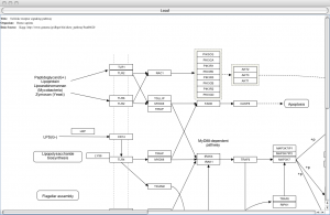
It’s a pretty simplistic example and doesn’t really allow much interactivity. But for my purposes, this is pretty useful. One downside of this approach is that it requires manually drawn pathways – so that they contain layout coordinates. As far as I can tell, only WikiPathways provides these, so displaying pathways from other sources is still problematic. A screen shot of a displayed pathway is below:


Viewing a pathway via the PathVisio classes

Viewing a pathway via the PathVisio classes

Plate Well Series Plots in R

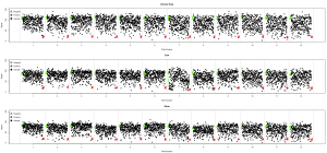
Plate well series plots are a common way to summarize well level data across multiple plates in a high throughput screen. An example can be seen in Zhang et al. As I’ve been working with RNAi screens, this visualization has been a useful way to summarize screening data and the various transformations on that data. It’s fundamentally a simple scatter plot, with some extra annotations. Though the x-axis is labeled with plate number, the values on the x-axis are actually well locations. The y-axis is usually the signal from that well.

Since I use it often, here’s some code that will generate such a plot. The input is a list of matrices or data.frames, where each matrix or data.frame represents a plate. In addition you need to specify a “plate map” – a character matrix indicating whether a well is a sample, (“c”) positive control (“p”), negative control (“n”) or ignored (“x”). The code looks like

1
2
3
4
5
6
7
8
9
10
11
12
13
14
15
16
17
18
19
20
21
22
23
24
25
26
plate.well.series <- function(plate.list, plate.map, draw.sep = TRUE, color=TRUE, ...) {
  signals <- unlist(lapply(plate.list, as.numeric))
  nwell <- prod(dim(plate.list[[1]]))
  nplate <- length(signals) / nwell

  cols <- 'black'
  if (color) {
    pcolor <- 'red'
    ncolor <- 'green'
    colormat <-  matrix(0, nrow=nrow(plate.list[[1]]), ncol=ncol(plate.list[[1]]))
    colormat[which(plate.map == 'n')] <- ncolor
    colormat[which(plate.map == 'p')] <- pcolor
    colormat[which(plate.map == 'c')] <-  'black'
    cols <- sapply(1:nwell, function(x) {
      as.character(colormat)
    })
  }
  plot(signals, xaxt='n', ylab='Signal', xlab='Plate Number', col = cols, ...)
  if (color) legend('topleft', bty='n', fill=c(ncolor, pcolor, 'black'),
                    legend=c('Negative', 'Positive', 'Sample'),
                    y.intersp=1.2)
  if (draw.sep) {
    for (i in seq(1, length(signals)+nwell, by=nwell)) abline(v=i, col='grey')
  }
  axis(side=1, at = seq(1, length(signals), by=nwell) + (nwell/2), labels=1:nplate)
}

An example of such a plot is below


Plate Well Series Plot

Plate well series plot


Another example comparing normalized data from three runs of an RNAi screen investigating drug sensitization (also highlighting the fact that plate 7 in the 5nm run was messed up):


Comparing runs with plate well series plots

Comparing runs with plate well series plots


From Theory to Practice

Some time back, John Van Drie and myself had done some work on characterizing structure-activity cliffs, which are molecules that have very similar structures but very different activities. The term originated from Maggiora, who suggested that this was a reason for the failure of many QSAR models. At the same time, such cliffs can represent the most interesting portions of a structure-activity relationship. Our first paper introduced the idea of the Structure Activity Landscape Index (SALI) – a numerical metric to characterize activity cliffs and SAR landscapes, and was followed by a paper describing how one could use SALI to characterize the quality of predictive models. We also put out some software to let others use SALI to analyse their own data.

A few weeks back I heard from Jinhua Zhang at Simulations Plus Inc., that they had implented the SALI methodology in their ADMET Predictor product. He also provided some slides showing how they used SALI to characterize a variety of predictive models for hERG inhibition.

It’s a nice feeling to see our theoretical work being incorporated into a real world product!

Hit Selection Methods for RNAi Screens

Over the last few weeks I’ve been getting up to speed on RNAi screening (see Lord et al for a nice overview) and one of the key features in this approach is to reliably select hits for followup. In many ways it is similar to hit selection in small molecule HTS but also employs techniques from the analysis of microarray data.

Very broadly, there are two types of selection methods: statistical and knowledge based. In general, one employs a statistical method first, possibly followed by triaging the initial list using a knowledge based method. As with small molecule HTS, true hits (true positives or TP) in general are the outliers, though it’s possible that assay artifacts will also look like true hits and these would be false positives (FP). But in general, the outliers are easy and the real challenge is with identifying moderately active siRNA’s (or compounds) as actual hits.

One can further divide statistical methods into ranking procedures or thresholding procedures. In the former one ranks the siRNA‘s by some metric and selects as many as can be followed up using available resources. In the latter, one identifies a threshold, above which any siRNA is regarded as a hit. One of the key features of many statistical methods is that they provide bounds on the FP and FN (false negative) rates. This is especially important with thresholding methods.

But what about siRNA‘s that lie just below the threshold? Should one ignore them? Is it possible to further investigate whether they might actually be hits? This is where a knowledge based approach can provide a second level of confirmation for false negatives or positives. This post summarizes recent work on hit selection in RNAi screens.

Statistical methods

Many statistical methods are similar to or derived from approaches employed in HTS experiments for small molecules. An excellent overview of statistical methods in HTS analysis is given by Malo et al and covers both assay quality metrics as well as hit selection methods.

One of the most common methods is to use a threshold of \(\mu \pm k \sigma\), where \(\mu\) and \(\sigma\) are the mean and standard deviation of the sample wells respectively and k is usually taken to be 3. This is also known as the z-score method, and assumes a normal distribution of signal values. However, in RNAi screens it’s not uncommon to have a number of extreme outliers. Such a situation would skew the mean based threshold to larger values, leading to fewer prospective hits being identified.

Instead, Zhang et al (as well as Chung et al) suggest the use of the \(median \pm 3 \textrm{MAD}\) method, where MAD is the mean absolute deviation and is given by

\(\textrm{MAD} = 1.4826\, median( | x_i – median(x) | ) \)

where \(x_i\) is the signal from well $\latex i$ and \(x\) represents all the sample wells. The key feature of this approach is that it is more robust to outliers and violations of the assumption that the signal data is normally distributed. Chung et al present a nice simulation study, highlighting the effectiveness of MAD based selection over mean based.

However, Zhang et al also note that the MAD method is not robust to skewed distributions. To address this they suggest a quartile based threshold method. For the sample data, one calculates the first, second and third quartiles (\(Q_1, Q_2, Q_3\)) and generates the lower and upper thresholds for hit selection as the smallest observed value just above \(Q_1 – c IQR\) and the largest observed value just below \(Q_3 – c IQR\) respectively. In both cases, \(IQR = Q_3 – Q_1\). A key feature of this method is the choice of \(c\), and is based on the desired targeted error rate (based on a normal distribution). Zhang et al show that one can choose \(c\) such that the resultant error rate is equivalent to that obtained from a mean or median-based thresholding scheme, for a given \(k\). Thus for \(k = 3\) in those methods, the quartile method would set \(c = 1.7239\).

In contrast to the above methods, which define a threshold and automatically select siRNA’s above the threshold as hits, one can order the wells using a metric and then simply select the top \(n\) wells for followup, where \(n\) is dictated by the resources available for followup. In this vein, Wiles et al discuss a variety of ranking metrics methods for RNAi screens. Some of the methods they discuss include simple background substraction quantile normalization and so on IQR normalization. Surprisingly, in their analysis, ranking of siRNA’s based on background subtraction outperformed IQR normalization.

Zhang et al (the Merck people have been busy!) described another ranking procedure based on the Strictly Standardized Mean Difference (SSMD) between signals from individual siRNA’s and a negative control. While conceptually similar to simple schemes such as percentage inhibition, this method is reported to be more robust to variability in the sample and control groups and also has a probabilistic interpretation. The latter aspect allowed the authors to develop a thresholding scheme, based on controlling the false positive and false negative rates.

Another approach described by Konig et al makes use of the fact that in RNAi screens, a given gene is targeted by 2 to 4 different siRNA’s. In contrast, none of the above methods, consider this aspect of an RNAi screen. Their method, termed RSA (redundant siRNA activity) analysis, initially ranks all wells in an assay based on their signals. Next, they consider the rank distribution of all siRNA’s targeting a given gene and determine a p-value, which indicates whether all the siRNA’s targeting a given gene have low ranks. They then rerank all wells based on their p-values , followed by their individual signals. The net result of this is that, even though a gene might have 4 wells (i.e., siRNA’s) exhibiting moderate activity (and so might be just below the threshold in a mean or MAD based analysis), it will be “weighted” more heavily than a gene with, say, just one highly active siRNA. Their experiments and analysis indicate that this is a useful method and their implementations (C#, Perl, R) are available. A nice side effect of this method is that they are able suggest an optimal (in terms of efficacy) number of redundant siRNA’s per gene.

Platewise or experimentwise?

One aspect that I haven’t mentioned is whether these analyses should be performed in a platewise manner or across all the plates in an experiment (i.e. experimentwise manner). Given that an RNAi screen can include a large number of plates, it’s possible that plate specific effects might skew an anaysis that considers all plates together. Thus platewise analysis can handle different systematic errors within plates. At the same time, a platwise analysis would be ignorant of any clustering that may be present amongst the hits, which would be identifiable is one performed the analysis in an experimentwise manner. Zhang et al suggest the following scheme, based on their observations that platewise analysis tends to have a higher probability of identifying true hits.

  • Select a thresholding method
  • Apply the method in an experimentwise manner on the normalized data, to see if hit clusters are present
  • If such clusters are present, repeat the above step on un-normalized data to check whether clustering is an artifact
  • If no clusters are observed, perform the analysis in a platewise manner and select hits from each plate

While a useful protocol, Zhang et al describe a Bayesian approach, derived from a similar method for microarray data (Newton et al). One of the key features of this approach is that it incorporates aspects of a platewise and experimentwise analysis in a single framework, obviating the need to choose one or the other.

Knowledge based methods

The statistics based methods work on the basis of relatively large samples and employ a variety of distributional assumptions. They’re certainly useful as a first pass filter, but various questions remain: Should we totally ignore wells that lie just below a threshold? Is there a way to check for false negatives? False positives?

To address these questions, before running a follow up screen, one can make use of external knowledge. More specifically, genes do not exist in isolation. Rather, they can be considered in terms of networks. Indeed, studies of PPI‘s (Chuang et al) and disease genes (Kohler et al) have suggested a guilt by association principle – genes that are close together in a network are more likely to exhibit similar functions or lead to similar phenotypes.

Wang et al employed this principle to characterize the genes targeted by siRNA’s in a screen, by constructing an interaction network (based on STRING data) and analyzing the connectivity of the genes from the screen in this context. Their observation was that genes corresponding to hits from the RNAi screen exhibited a higher degree of connectivity, compared to random networks. While an interesting approach, some of it does seem a little ad hoc. Given the fact that it depends on PPI data, the networks constructed from screening results may be incomplete, if the PPI database does not contain interactions for the genes in question. In addition, while their network based scoring method seems to correlate somewhat with followup results, it’s not very consistent. However, the approach makes sense and correctly catches false negatives in their test cases. Their R code for the network based scoring system is available.

Interestingly, I haven’t found many other studies of such knowledge based hit selection methods. While networks are one way to identify related genes, other methods could be considered and it would be interesting to see how they compare.
R and Oracle

It’s been a while since my last post, but I’m getting up to speed at work. It’s been less than a month, but there’s already a ton of cool stuff going on. One of the first things I’ve been getting to grips with is the data infrastructure at the NCGC, which is based around Oracle. One of my main projects is handling informatics for RNAi screening. As the data comes out of the pilots, they get loaded into the Oracle infrastructure.

Being an R aficionado, I’m doing the initial, exploratory analyses (normalization, hit selection, annotation etc.) using R. Thus I needed to have a way to access an Oracle DB from R. This is supported by the ROracle package. But it turns out that the installation is a little non-obvious and I figured I’d describe the procedure (on OS X 10.5) for posterity.

The first thing to do is to get Oracle from here. Note that this is the full Oracle installation and while it comes with 32 bit and 64 bit libraries, some of the binaries that are required during the R install are 64 bit only. After getting the zip file, extract the installation files and run the installation script. Since I just needed the libraries (as opposed to running an actual Oracle DB), I just went with the defaults and opted out of the the actual DB creation step. After installation is done, it’s useful to set the following environment variables:

1
2
3
export ORACLE_HOME=/Users/foo/oracle
export LD_LIBRARY_PATH=$ORACLE_HOME/lib:$LD_LIBRARY_PATH
export DYLD_LIBRARY_PATH=$ORACLE_HOME/lib:$DYD_LIBRARY_PATH

With Oracle installed, execute the following

1
$ORACLE_HOME/bin/genclntst

This will link a variety of object files into a library, which is required by the R package, but doesn’t come in the default Oracle installation.

The next thing is to get a 64 bit version of R from here and simply install as usual. Note that this will require you to reinstall all your packages, if you had a previous version of R around. Specifically, before installing ROracle, make sure to install the DBI package.

After installing R, get the ROracle 0.5-9 source package. Since there’s no binary build for OS X, we have to compile it ourselves. Before building, I like to CHECK the package to make sure that all is OK. Thus, the sequence of commands is

1
2
3
4
tar -zxvf ROracle_0.5-9.tar.gz
R --arch x86_64 CMD CHECK ROracle
R --arch x86_64 CMD BUILD ROracle
R --arch x86_64 CMD INSTALL -l  /Users/guhar/Library/R/2.9/library ROracle_0.5-9.tar.gz

When I ran the CHECK, I did get some warnings, but it seems to be safe to ignore them.

At this stage, the ROracle package should be installed and you can start R and load the package. Remember to start R with the –arch x86_64 argument, since the ROracle package will have been built for the 64 bit version of R.