At work, a colleague gave an interesting presentation on characterizing associations between continuous and categorical variables. I expect that I will be facing this issue in some upcoming work so was doing a little reading and made some notes for myself.

Given a continuous variable Y and a categorical variable G, is the distribution of Y independent of the levels of G? One can address this using parametric or non-parametric methods. Due to the superior power of parametric methods we start by considering them and only if we completely fail to satisfy the distributional assumptions of such methods, do we move to the non-parametric methods.

A simple approach is to convert G to an indicator variable matrix, such that each level of G becomes a binary vector, and then use this matrix and Y to fit a linear model. One can then perform an ANOVA on the fit to check whether Y is independent of the groups. This approach assumes that Y is normally distributed, and that variances are equal amongst the groups.

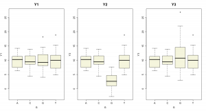
A simple example in R is as follows. We first create a dataset in which there is no difference in the mean or variance across the groups, one in which the means differ and one in which the variances differ

A summary of the Y’s grouped by G are given below.

We now run the ANOVA, using the first dataset.

Running this gives us

If we consider the 0.05 significance level, we would not reject the null hpothesis that Y is independent of G. If we now rerun the ANOVA using the second dataset

we get

which suggests that we reject the null hypothesis and accept the alternative that there is the Y’s are not independent of the groups (which is true by design).

Furthermore, it really only indicates whether there is a dependence between the groups and the means of the group members – it doesn’t tell us anything about lack of independence in terms of scale parameters. This is not surprising since the linear model is defined to have a constant variance. Thus, if we want to investigate dependence of the variance on groups, we should look at distributions of residuals or other approaches to identifying heteroscedacity (such as Levenes test).

In case we cannot satisfy the assumptions (even after investigating possible transformations of the data) required for ANOVA, we can move to parametric methods, which are easy to run, but have a lower power. For this problem, the Kruskal-Wallis test and the Fligner-Killeen test come in handy. These methods are in the base stats package but also come with the coin package which is handy for running a variety of independence tests.

The Kruskal-Wallis test makes no assumptions about normality, but does assume that the distributions amongst the levels of G are of the same shape and have the same variance (and so, the differences are due to differences in the means). The Fligner-Killeen test also avoids the normality assumption bu in this case, has the null hypothesis that the variances in the groups are the same. Thus ideally, we’d run the Kruskal-Wallis first and if we could not reject the null hypothesis we then investigate whether there is a difference in the variances across the groups by the Fligner-Killeen tests.

Some examples highlight the analysis. First, we consider the dataset that is independent of the groups (Y1):

which indicates that we fail to reject the null hypothesis that the distribution of Y1 is independent of the levels of G. We then consider the dataset where the means are dependent on the groups

which indicates the we can reject the null hypothesis. However, note that for Y3, where the means are independent of the groups but the variance differ, the Kruskal-Wallis test is not useful:

On the other hand, if we run the Fligner-Killeen test on these three datasets, we correctly identify Y3 as having its variance dependent on G