Differential Dose Response – Some More Exploration

This is a follow on to my previous post that described a recent paper where we explored a few ways to characterize the differential activity of small molecules in dose response screens. In this post I wanted to highlight some aspects of this type of analysis that didn’t make it into the final paper.

TL;DR there’s more to differential analysis of dose response data than thresholding and ranking.

Comparing Model Fits

One approach to characterizing differential activity is to test whether the curve fit models (in our case 4-parameter Hill models) are indistinguishable or not. While traditionally, ANOVA could be used to test this, it assumes that the models being compared are nested. This is not the case when testing for effects of different treatments (i.e., same model, but different datasets). As a result we first considered the use of AIC – but even then, applying this to the same model built on different datasets is not really valid.

Another approach (described by Ritz et al) that we considered was to refit the curves for the two treatments simultaneously using replicates, and determines whether the ratio of the AC50’s (termed the Selectivity Index or SI) from the two models was different from 1.0. We can then test the hypothesis and determine whether the SI was statistically significant or not. The drawback is that it, ideally, requires that the curves differ only in potency. In practice this is rarely the case as effects such as toxicity might cause a shift the in the response at low concentrations, partial efficacy might cause incomplete curves at high concentrations and so on.

simufit1 
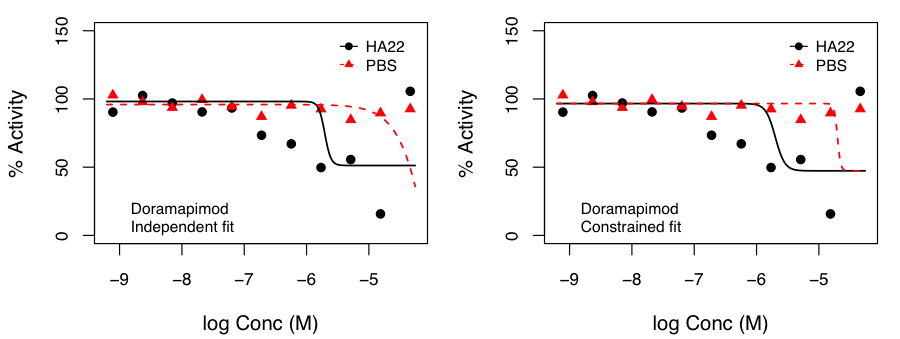
We examined this approach by fitting curves such that the top and bottom of the curves were constrained to be identical in both treatments and only the Hill slope and AC50 were allowed to vary.

After, appropriate correction, this identified molecules that exhibited p < 0.05 for the hypothesis thatsimufit2 
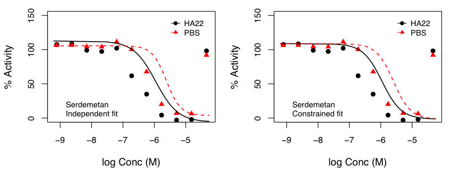
the SI was not 1.0. Independent and constrained curve fits for two compounds are shown alongside. While the constraint of equal top and bottom for both curves does lead to some differences compared to independent fits (especially from the point of view of efficacy), the current data suggests that the advantage of such a constraint (allowing robust inference on the statistical significance of SI) outweighs the disadvantages.

Variance Stabilization

Finally, given the rich literature on differential analysis for genomic data, our initial hope was to simply apply methods from that domain to the current problems. However, variance stabilization becomes an issue when dealing with small molecule data. It is well known from gene expression experiments that that the variance in replicate measurements can be a function of the mean value of the replicates. If not taken into account, this can mislead a t-test into identifying a gene (or compound, in our case) as exhibiting non-differential behavior, when in fact it is differentially expressed (or active).

The figure below compares the standard deviation (SD) versus mean of each compound, for each parameter in the two treatments (HA22, an immunotoxin and PBS, the vehicle treatment). Overlaid on the scatter plot is a loess fit. In the lower panel, we see that in the PBS treatment there is minimal dependency of SD on the mean values, except for the case of log AC50. However, for the case of HA22 treatment, each parameter shows a distinct dependence of SD on the mean replicate value.

vsn1 vsn2

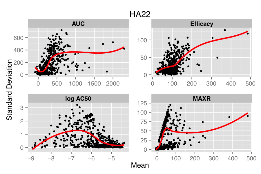
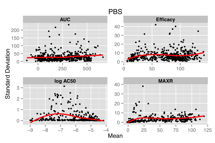
Many approaches have been designed to address this issue in genomic data (e.g., Huber et al, Durbin et al, Papana & Ishwaran). One of the drawbacks of most approaches is that they assume a distributional model for the errors (which in the case of the small molecule data would correspond to the true parameter value minus the calculated value) or a specific model for the mean-variance relationship. However, to our knowledge, there is no general solution to the problem of choosing an appropriate error distribution for small molecule activity (or curve parameter) data. A non-parametric approach described by Motakis et al employs the observed replicate data to stabilize the variance, avoiding any distributional assumptions. However, one requirement is that the mean-variance relationship be monotonic increasing. From the figure above we see that this is somewhat true for efficacy but does not hold, in a global sense, for the other parameters.

Overall, differential analysis of dose response data is somewhat of an open topic. While simple cases of pure potency or efficacy shifts can be easily analyzed, it can be challenging when all four curve fit parameters change. I’ve also highlighted some of the issues with applying methods devised for genomic data to small molecule data – solutions to these would enable the reuse of some powerful machinery.

Analysing Differential Activity in Dose Response Screens

My colleagues and I recently published a paper where we explored a few methods to identify differential behavior in dose response screens. While there is an extensive literature about analyzing differential effects in genomic data (e.g. mciroarrays, RNAseq), these methods are based on distributional assumptions that holds for genomic data. This is not necessarily the case for small molecule, dose response data. A separate post will explore this aspect.

So we couldn’t directly apply the methods devised for genomic data. Another issue that we wanted to address was the lack of replicates. As a result certain methods are excluded from consideration (e.g., t-test based methods). The simplest case (or what we refer to as obviously differential) is when a compound is active in one treatment and completely inactive in the other. This is trivial to characterize. The next method we considered was to look at fold changes for individual curve fit parameters and then choose an arbitrary threshold. This is not a particularly robust approach, and has no real statistical basis. However, such thresholding is still used in a number of scenarios (e.g., cherry picking in single point screens). In addition, in this approach you have to choose one of many parameters. So finally, we considered a data fusion approach, that ranked compounds using the rank product method. This method employed potency, response at the highest concentration and the AUC. The nice thing about this method is that it doesn’t require choosing a threshold, provides an empirical p-value and is flexible enough to include other relevant parameters (say, physicochemical properties).

Finally, we examined how single point data (modeled using the response at the highest concentration) compared to dose response data at identifying differential actives. As one might expect, the obviously differential compounds were easily identified. However for compounds active in both treatments, the single point approach led to more false positives. Thus, even those dose response is more resource-intensive, the improved accuracy makes it worth it.

In the next post I’ll look at some of the issues that didn’t make in to this paper – in particular hypothesis based tests that focus on testing differences between model fits. One key observation (also suggested by Gelman) is that strict p-value cutoffs lead one to focus on obvious or well-known effects. For small-scale exploratory analyses such as described in this paper, a more relaxed threshold of 0.1 might be more suitable, allowing marginal effects that may, however, be biologically interesting to be considered.

Call For Papers: Shedding Light on the Dark Genome – Methods, Tools & Case Studies

252nd ACS National Meeting
Philadelphia, Aug 21-25, 2016
CINF Division

Dear Colleagues, we are organizing a symposium at the Fall ACS meeting in Philadelphia focusing on computational, experimental and hybrid approaches to characterizing the unstudied and understudied druggable genome.  In 2014 the NIH initiated a program titled, “Illuminating the Druggable Genome” (IDG) with the goal of improving our understanding of the properties and functions of proteins that are currently unannotated within the four most commonly drug-targeted protein families – GPCRs, ion channels, nuclear receptors and kinases. As part of this program a Knowledge Management Center (KMC) was formed, as a collaboration between six academic center, who’s goal was to develop an integrative informatics platform to collect data, develop data driven prioritization schemes, analytical methods  and disseminate standardized/annotated information related to the unannotated proteins in the four gene families of interest.

In this symposium, members of the various components of the IDG program will present the results of ongoing work related to experimental methods, target prioritization, data aggregation and platform development. In addition, we welcome contributions related to the identification of druggable targets, approaches to quantify druggability and novel approaches to integrating disparate data source with the goal of shedding light on the “dark genome”

The deadline for abstract submissions is March 29, 2016. All abstracts should be submitted via MAPS at http://bit.ly/1mMqLHj. If you have any questions feel free to contact  Tudor or myself

Rajarshi Guha
NCATS, NIH
guhar@mail.nih.gov

Tudor Oprea
University of New Mexico
TOprea@salud.unm.edu

vSDC, Rank Products and DUD-E

This post is a follow-up to my previous discussion on a paper by Chaput et al. The gist of that paper was that in a virtual screening scenario where a small number of hits are to be selected for followup, one could use an ensemble of docking methods, identify compounds whose scores were beyond 2SD of the mean for each method and take the intersection. My post suggested that a non-parametric approach (rank products, RP) performed similarly to the parametric approach of Chaput et al on the two targets they screened.

The authors also performed a benchmark comparison of their consensus method (vSDC) versus the individual docking methods for 102 DUD-E targets. I was able to obtain the individual docking scores (Glide, Surflex, FlexX and GOLD) for each of the targets, with the aim of applying the rank product method described previously.

In short, I reproduced Figure 6A (excluding the curve for vSDC). In
th0this figure, \(n_{test}\) is the number of compounds selected (from the ranked list, either by individual docking scores or by the rank product) and \(T_{h>0}\) is the percentage of targets for which the \(n_{test}\) selected compounds included one or more actives. Code is available here, but you’ll need to get in touch with the authors for the DUD-E docking scores.

As shown alongside, the RP method (as expected) outperforms the individual docking methods. And visual comparison with the original figure suggests that it also outperforms vSDC, especially at lower values of \(n_{test}\). While I wouldn’t regard the better performance of RP compared to vSDC as a huge jump, the absence of a threshold certainly works in its favor.

One could certainly explore ranking approaches in more depth. As suggested by Abhik Seal, Borda or Condorcet methods could be examined (though the small number of docking methods, a.k.a., voter, could be problematic).

UPDATE: After a clarification from Liliane Mouawad it turns out there was a mistake in the ranking of the Surflex docking scores. Correcting that bug fixes my reproduction of Figure 6A so that the curves for individual docking methods match the original. But more interestingly, the performance of RP is now clearly better than every individual method and the vSDC method as well, at all values of \(n_{test}\)

Hit Selection When You’re Strapped for Cash

I came across a paper from Chaput et al that describes an approach to hit selection from a virtual screen (using docking), when follow-up resources are limited (a common scenario in many academic labs). Their approach is based on using multiple docking programs. As they (and others) have pointed out, there is a wide divergence between the rankings of compounds generated using different programs. Hence the motivation for a consensus approach, based on the estimating the standard deviation (SD) of scores generated by a given program and computing the intersection of compounds whose scores are greater than 2 standard deviations from the mean, in each program. Based on this rule, they selected relatively few compounds – just 14 to 22, depending on the target and confirmed at least one of them for each target. This represents less than 0.5% of their screening deck.

However, their method is parametric – you need to select a SD threshold. I was interested in seeing whether a non-parametric, ranking based approach would allow one to retrieve a subset that included the actives identified by the authors. The method is essentially the rank product method applied to the docking scores. That is, the compounds are ranked based on their docking scores and the “ensemble rank” for a compound is the product of its ranks according to each of the four programs. In contrast to the original definition, I used a sum log rank to avoid overflow issues. So the ensemble rank for the \(i\)’th compound is given by

\(R_i = \sum_{j=1}^{4} \log r_{ij}\)

where \(r_{ij}\) is the rank of the \(i\)’th compound in the \(j\)’th docking program. Compounds are then selected based on their ensemble rank. Obviously this doesn’t give you a selection per se. Instead, this allows you to select as many compounds as you want or need. Importantly, it allows you to introduce external factors (cost, synthetic feasibility, ADME properties, etc.) as additional rankings that can be included in the ensemble rank.

Using the docking scores for Calcineurin and Histone Binding Protein (Hbp) provided by Liliane Mouawad (though all the data really should’ve been included in the paper) I applied this method using the code below

1
2
3
4
5
6
7
8
9
10
library(stringr)
d <- read.table('http://cmib.curie.fr/sites/u759/files/document/score_vs_cn.txt',
                header=TRUE, comment='')
names(d) <- c('molid', 'Surflex', 'Glide', 'Flexx', 'GOLD')
d$GOLD <- -1*d$GOLD ## Since higher scores are better
ranks <- apply(d[,-1], 2, rank)
lranks <- rowSums(log(ranks))
tmp <- data.frame(molid=d[,1], ranks, lrp=rp)
tmp <- tmp[order(tmp$lrp),]
which(str_detect(tmp$molid, 'ACTIVE'))

and identified the single active for Hbp at ensemble rank 8 and the three actives for Calcineurin at ranks 3, 5 and 25. Of course, if you were selecting only the top 3 you would’ve missed the Calcineurin hit and only have gotten 1/3 of the HBP hits. However, as the authors nicely showed, manual inspection of the binding poses is crucial to making an informed selection. The ranking is just a starting point.

Update: Docking scores for Calcineurin and Hbp are now available