Which Datasets Lead to Predictive Models?

I came across a recent paper from the Tropsha group that discusses the issue of modelability – that is, can a dataset (represented as a set of computed descriptors and an experimental endpoint) be reliably modeled. Obviously the definition of reliable is key here and the authors focus on a cross-validated classification accuracy as the measure of reliability. Furthermore they focus on binary classification. This leads to a simple definition of modelability – for each data point, identify whether it’s nearest neighbor is in the same class as the data point. Then, the ratio of number of observations whose nearest neighbor is in the same activity class to the number observations in that activity class, summed over all classes gives the MODI score. Essentially this is a statement on linear separability within a given representation.

The authors then go show a pretty good correlation between the MODI scores over a number of datasets and their classification accuracy. But this leads to the question – if one has a dataset and associated modeling tools, why compute the MODI? The authors state

we suggest that MODI is a simple characteristic that can be easily computed for any dataset at the onset of any QSAR investigation

I’m not being rigorous here, but I suspect for smaller datasets the time requirements for MODI calculations is pretty similar to building the models themselves and for very large datasets MODI calculations may take longer (due to the requirement of a distance matrix calculation – though this could be alleviated using ANN or LSH). In other words – just build the model!

Another issue is the relation between MODI and SVM classification accuracy. The key feature of SVMs is that they apply the kernel trick to transform the input dataset into a higher dimensional space that (hopefully) allows for better separability. As a result MODI calculated on the input dataset should not necessarily be related to the transformed dataset that is actually operated on by the SVM. In other words a dataset with poor MODI could be well modeled by an SVM using an appropriate kernel.

The paper, by definition, doesn’t say anything about what model would be best for a given dataset. Furthermore, it’s important to realize that every dataset can be perfectly predicted using a sufficiently complex model. This is also known as an overfit model. The MODI approach to modelability avoids this by considering a cross-validated accuracy measure.

One application of MODI that does come to mind is for feature selection – identify a descriptor subset that leads to a predictive model. This is justified by the observed correlation between the MODI scores and the observed classification rates and would avoid having to test feature subsets with the modeling algorithm itself. An alternative application (as pointed out by the authors) is to identify subsets of the data that exhibit a good MODI score, thus leading to a local QSAR model.

More generally, it would be interesting to extend the concept to regression models. Intuitively, a dataset that is continuous in a given representation should have a better modelability than one that is discontinuous. This is exactly the scenario that can be captured using the activity landscape approach. Sometime back I looked at characterizing the roughness of an activity landscape using SALI and applied it to the feature selection problem – being able to correlate such a measure to predictive accuracy of models built on those datasets could allow one to address modelability (and more specifically, what level of continuity should a landscape present to be modelable) in general.

fingerprint 3.5.2 released

Comparison of nested loop performance in R and C for Tanimoto similarity matrix calculation.

Comparison of nested loop performance in R and C for Tanimoto similarity matrix calculation.

Version 3.5.2 of the fingerprint package has been pushed to CRAN. This update includes a contribution from Abhik Seal that significantly speeds up similarity matrix calculations using the Tanimoto metric.

His patch led to a 10-fold improvement in running time. However his code involved the use of nested for loops in R. This is a well known bottleneck and most idiomatic R code replaces for loops with a member of the sapply/lapply/tapply family. In this case however, it was easier to write a small piece of C code to perform the loops, resulting in a 4- to 6-fold improvement over Abhiks observed running times (see figure summarizing Tanimoto similarity matrix calculation for 1024 bit fingerprints, with 256 bits randomly selected to be 1). As always, the latest code is available on Github.

Exploring co-morbidities in medical case studies

A previous post described a first look at the data available in casesdatabase.com, primarily looking at summaries of high level meta-data. In this post I start looking at the cases themselves. As I noted previously, BMC has performed some form of biomedical entity recognition on the abstracts (?) of the case studies, resulting in a set of keywords for each case study. The keywords belong to specific types such as Condition, Medication and so on. The focus of this post will be to explore the occurrence of co-morbidities – which conditions occur together, to what extent and whether such occurrences are different from random. The code to extract the co-morbidity data and generate the analyses below is available in co-morbidity.py

Before doing any analyses we need to do some clean up of the Condition keywords. This includes normalizing terms (replacing ‘comatose’ with ‘coma’, converting all diabetes variants such as Type 1 and Type 2 to just diabetes), fixing spelling variants (replacing ‘foetal’ with ‘fetal’), removing stopwords and so on. The Python code to perform this clean up requires that we manually identify these transformations. I haven’t done this rigorously, so it’s not a totally cleansed dataset. The cleanup code looks like

1
2
3
4
5
6
7
8
9
10
11
12
13
14
15
16
17
18
19
20
21
22
23
24
25
26
27
28
def cleanTerms(terms):
    repMap = {'comatose':'coma',
              'seizures':'seizure',
              'foetal':'fetal',
              'haematomas':'Haematoma',
              'disorders':'disorder',
              'tumour':'tumor',
              'abnormalities':'abnormality',
              'tachycardias':'tachycardias',
              'lymphomas': 'lymphoma',
              'tuberculosis':'tuberculosis',
              'hiv':'hiv',
              'anaemia':'anemia',
              'carcinoma':'carcinoma',
              'metastases':'metastasis',
              'metastatic':'metastasis',
              '?':'-'}
    stopwords = ['state','syndrome'', low grade', 'fever', 'type ii', 'mellitus', 'type 2', 'type 1', 'systemic', 'homogeneous', 'disease']
    l = []
    term = [x.lower().strip() for x in terms]
    for term in terms:
        for sw in stopwords: term = term.replace(sw, '')
        for key in repMap.keys():
            if term.find(key) >= 0: term = repMap[key]
        term = term.encode("ascii", "ignore").replace('\n','').strip()
        l.append(term)
    l = filter(lambda x: x != '-', l)
    return(list(set(l)))

Since each case study can be associated with multiple conditions, we generate a set of unique condition pairs for each case, and collect these for all 28K cases I downloaded previously.

1
2
3
4
5
6
7
8
9
10
cases = pickle.load(open('cases.pickle'))
allpairs = []
for case in cases:
    ## get all conditions for this case
    conds = filter(lambda x: x['type'] == 'Condition', [x for x in case['keywords']])
    conds = cleanTerms([x['text'] for x in conds])
    if len(conds) == 0: continue
    conds.sort()
    pairs = [ (x,y) for x,y in list(combinations(conds, 2))]
    allpairs.extend(pairs)

It turns out that across the whole dataset, there are a total of 991,466 pairs of conditions corresponding to 576,838 unique condition pairs and 25,590 unique conditions. Now, it’s clear that some condition pairs may be causally related (some of which are trivial cases such as cough and infection), whereas others are not. In addition, it is clear that some condition pairs are related in a semantic, rather than causal, fashion – carcinoma and cancer. In the current dataset we can’t differentiate between these classes. One possibility would be to code the conditions using ICD10 and collapse terms using the hierarchy.

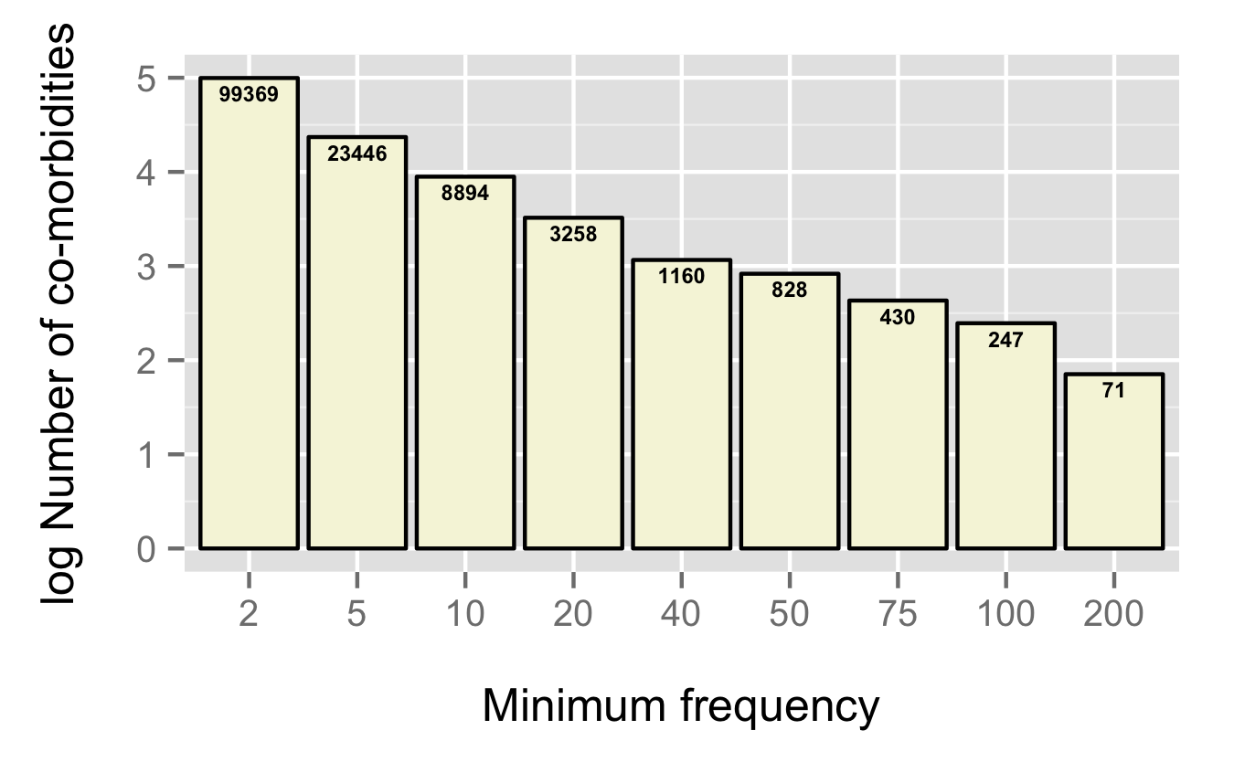
Number of co-morbidities vs frequency of occurrence

Number of co-morbidities vs frequency of occurrence

Having said that, we work with what we currently have – and it’s quite sparse. In fact the 28K case studies represent just 0.16% of all possible co-morbidities. Within the set of just under 600K unique observed co-morbidities, the bulk occur just once. For the rest of the analysis we ignore these singleton co-morbidities (leaving us with 513,997  co-morbidities). It’s interesting to see the distribution of frequencies of co-morbidities. The first figure plots the number of co-morbidities that occur at least N times – 99,369 co-morbidities occur 2 or more times in the dataset and so on.

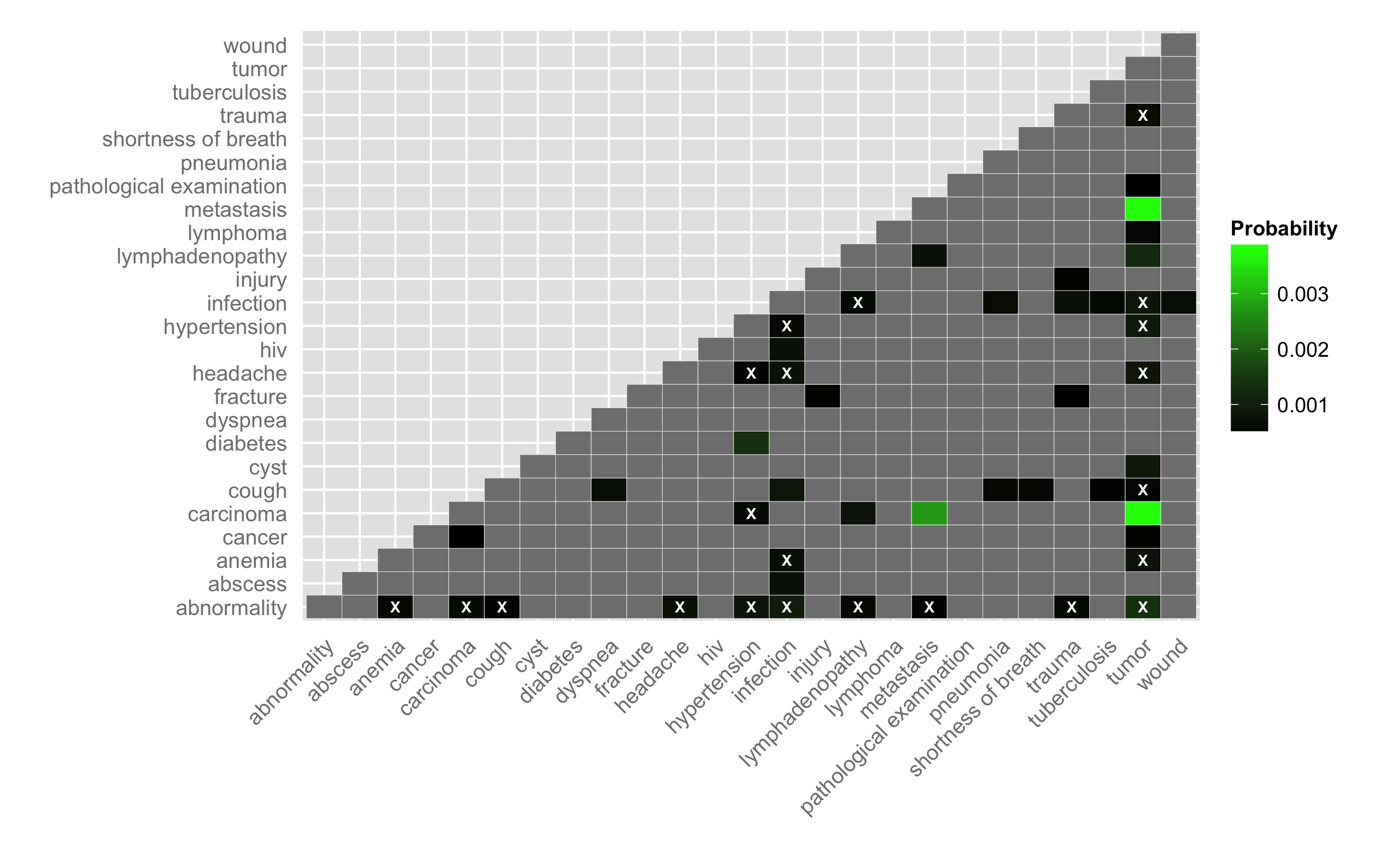
Another way to visualize the data is to plot a pairwise heatmap of conditions. For pairs of conditions that occur in the cases dataset we can calculate the probability of occurrence (i.e., number of times the pair occurs divided by the number of pairs). Furthermore, using a sampling procedure we can evaluate the number of times a given pair would be selected randomly from the pool of conditions. For the current analysis, I used 1e7 samples and evaluated the probability of a co-morbidity occurring by chance. If this probability is greater than the observed probability I label that co-morbidity as not different from random (i.e., insignificant). Ideally, I would evaluate a confidence interval or else evaluate the probability analytically (?).

For the figure below, I considered the 48 co-morbidities (corresponding to 25 unique conditions) that occurred 250 or more times in the dataset. I display the lower triangle for the heatmap – grey indicates no occurrences for a given co-morbidity and white X’s identify co-morbidities that have a non-zero probability of occurrence but are not different from random. As noted above, some of these pairs are not particularly informative – for example, tumor and metastasis occur with a relatively high probability, but this is not too surprising

Probability of occurrence for co-morbidities occurring more than 250 times

Probability of occurrence for co-morbidities occurring more than 250 times

It’s pretty easy to modify co-morbidity.py to look at other sets of co-morbidities. Ideally, however, we would precompute probabilities for all co-morbidities and then support interactive visualization (maybe using D3).

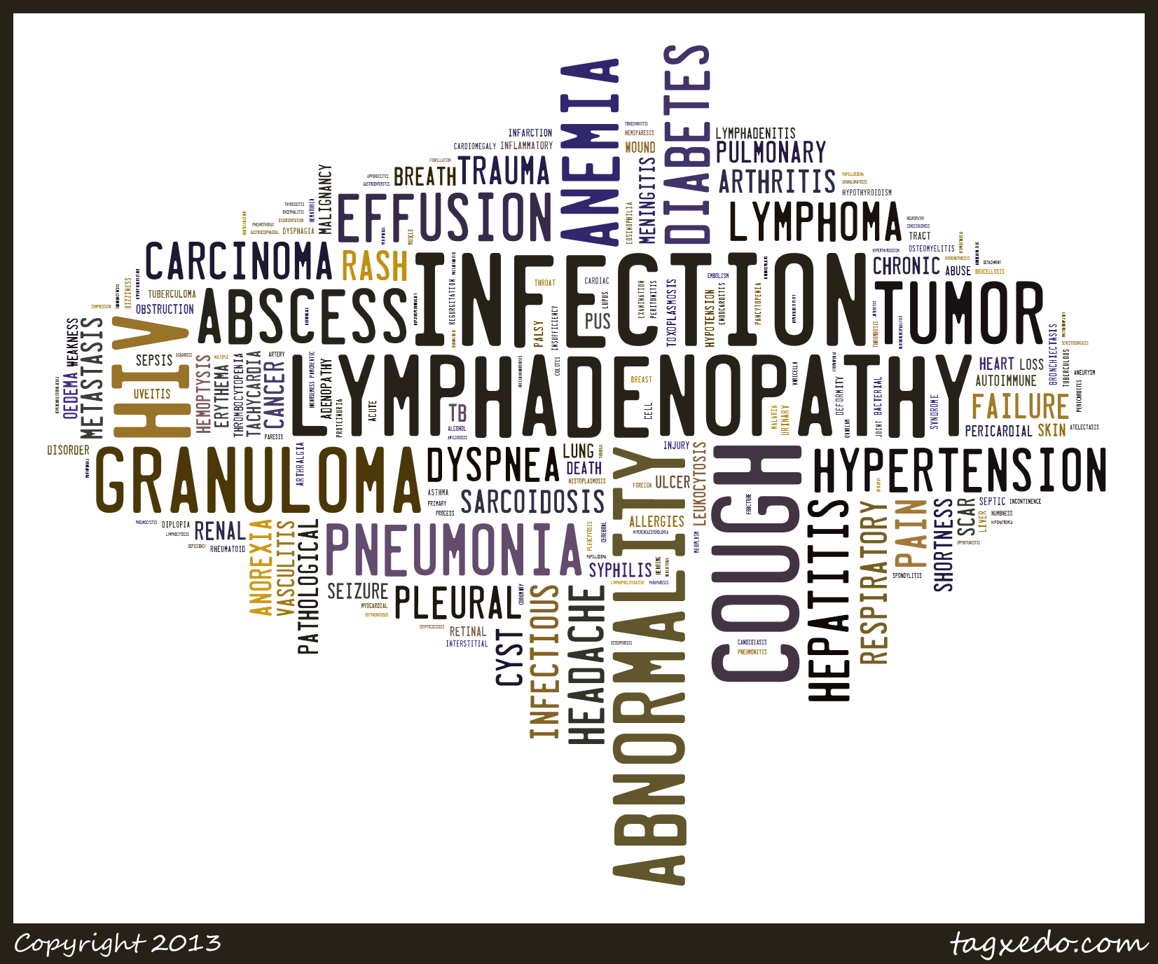
It’s also interesting to look at co-morbidities that include a specific condition. For example, lets consider tuberculosis (and all variants). There are 948 unique co-morbidities that include tuberculosis as one of the conditions. While the bulk of them occur just twice, there are a number with relatively large frequencies of occurrence – lymphadenopathy co-occurs with tuberculosis 203 times. Rather than tabulate the co-occurring conditions, we can use the frequencies to generate a word cloud, as shown below. As with the co-morbidity heatmaps, this could be easily automated to support interactive exploration. On a related note, it’d be quite interesting to compare the frequencies discussed here with data extracted from a live EHR system

A visualization of conditions most frequently co-occurring with tuberculosis

A visualization of conditions most frequently co-occurring with tuberculosis

So far this has been descriptive – given the size of the data, we should be able to try out some predictive models. Future posts will look at the possibilities of modeling the case studies dataset.

Exploring medical case studies

I recently came across http://www.casesdatabase.com/ from BMC, a collection of more than 29,000 peer-reviewed case studies collected from a variety of journals. I’ve been increasingly interested in the possibilities of mining clinical data (inspired by impressive work from Atul Butte, Nigam Shah and others), so this seemed like a great resource to explore

The folks at BMC have provided a REST API, which is still in development – as a result, there’s no public documentation and it still has a few rough edges. However, thanks to help from Demitrakis Kavallierou, I was able to interact with the API and extract summary search information as well as 28,998 case studies as of Sept 23, 2013. I’ve made the code to extract case studies available as proc.py. Running this, gives you two sets of data.

  1. A JSON file for each year between 2000 and 2014, containing the summary results for all cases in that year which includes a summary view of the case, plus facets for a variety of fields (age, condition, pathogen, medication, intervention etc.)
  2. A pickle file containing the case reports, as a list of maps. The case report contains the full abstract, case report identifier and publication meta-data.

A key feature of the case report entries is that BMC has performed some form of entity recognition so that it provides a list of keywords identified by different types: ‘Condition’, ‘Symptom’, ‘Medication’ etc. Each case may have multiple occurences for each type of keyword and importantly, each keyword is associated with the text fragment it is extracted from. As an example consider case 10.1136/bcr.02.2009.1548. The entry extracts two conditions

1
2
3
{u'sentence': u'She was treated by her family physician for presumptive interscapular myositis with anti-inflammatory drugs, cold packs and rest.',
u'text': u'Myositis',
u'type': u'Condition'}

and

1
2
3
{u'sentence': u'The patient denied any constitutional symptoms and had no cough.',
u'text': u'Cough',
u'type': u'Condition'}

I’m no expert in biomedical entity recognition, but the fact that BMC has performed it, saves me from having to become one, allowing me to dig into the data. But there are the usual caveats associated with text mining – spelling variants, term variants (insulin and insulin therapy are probably equivalent) and so on.

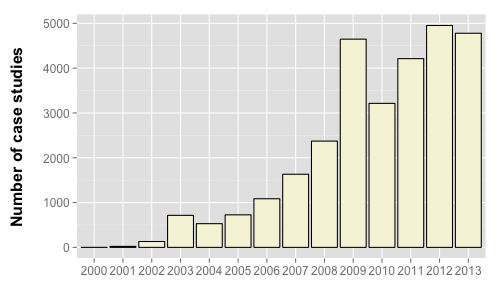
Count of cases deposited per year

Count of cases deposited per year

However, before digging into the cases themselves, we can use the summary data, and especially the facet information (which is, by definition, standardized) to get some quick summaries from the database. For example we see the a steady increase of case studies deposited in the literature over the last decade or so.

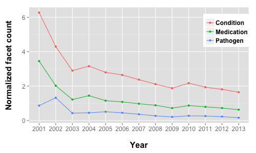
Interestingly, the number of unique conditions, medications or pathogens reported for these case studies is more or less constant, though there seems to be a downward trend for conditions. The second graph highlights this trend, by plotting the number of unique facet terms (for three types of facets) per year, normalized by the number of cases deposited that year.

Normalized count of unique facet terms by year

Normalized count of unique facet terms by year

This is a rough count, since I didn’t do any clean up of the text – so that misspellings of the same term (say, acetaminophen and acetaminaphen will be counted as two separate medication facets) may occur.

Another interesting task would be to enrich the dataset with additional annotations – ICD9/ICD10 for conditions, ATC for drugs – which would allow a higher level categorization and linking of case studies. In addition, one could use the CSLS service to convert medication names to chemical structures and employ structural similarity to group case studies.

The database also records some geographical information for each case. Specifically, it lists the countries that the authors are from. While interesting to an extent, it would have been nice if the country of occurrence or country of treatment were specifically extracted from the text. Currently, one might infer that the treatment occurred in the same country as the author is from, but this is likely only true when all authors are from the same country. Certainly, multinational collaborations will hide the true number of cases occurring in a given country (especially so for tropical diseases).

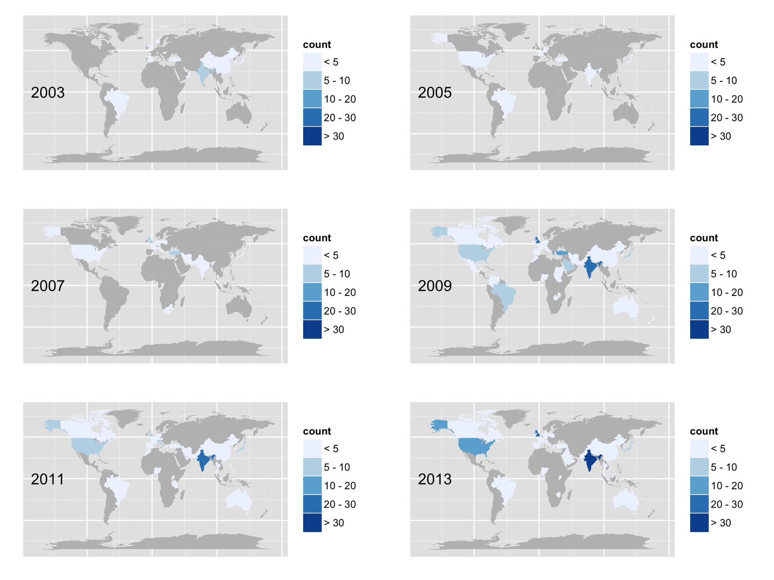
But we can take a look at how the number of cases reported for specific conditions, varies with geography and time. The figure below shows the cases whose conditions included the term tuberculosis

Tuberculosis cases by country and year

Tuberculosis cases by country and year

The code to extract the data from the pickle file is in condition_country.py. Assuming you have cases.pickle in your current path, usage is

1
$ python condition_country.py condition_name

and will output the data into a CSV file, which you can the process using your favorite tools.

In following blog posts, I’ll start looking at the actual case studies themselves. Interesting things to look at include exploring the propensity of co-morbidities, analysing the co-occurrence of conditions and medications or conditions and pathogens, to see whether the set of treatments associated with a given condition (or pathogen) has changed over time. Both these naturally lead to looking at the data with eye towards repurposing events.

Updated version of rcdk (3.2.3)

I’ve pushed updates to the rcdklibs and rcdk packages that support cheminformatics in R using the CDK. The new versions employ the latest CDK master, which as Egon pointed out  has significantly fewer bugs, and thanks to Jon, improved performance. New additions to the package include support for the LINGO and Signature fingerprinters (you’ll need the latest version of fingerprint).