A previous post described a first look at the data available in casesdatabase.com, primarily looking at summaries of high level meta-data. In this post I start looking at the cases themselves. As I noted previously, BMC has performed some form of biomedical entity recognition on the abstracts (?) of the case studies, resulting in a set of keywords for each case study. The keywords belong to specific types such as Condition, Medication and so on. The focus of this post will be to explore the occurrence of co-morbidities – which conditions occur together, to what extent and whether such occurrences are different from random. The code to extract the co-morbidity data and generate the analyses below is available in co-morbidity.py

Before doing any analyses we need to do some clean up of the Condition keywords. This includes normalizing terms (replacing ‘comatose’ with ‘coma’, converting all diabetes variants such as Type 1 and Type 2 to just diabetes), fixing spelling variants (replacing ‘foetal’ with ‘fetal’), removing stopwords and so on. The Python code to perform this clean up requires that we manually identify these transformations. I haven’t done this rigorously, so it’s not a totally cleansed dataset. The cleanup code looks like

Since each case study can be associated with multiple conditions, we generate a set of unique condition pairs for each case, and collect these for all 28K cases I downloaded previously.

It turns out that across the whole dataset, there are a total of 991,466 pairs of conditions corresponding to 576,838 unique condition pairs and 25,590 unique conditions. Now, it’s clear that some condition pairs may be causally related (some of which are trivial cases such as cough and infection), whereas others are not. In addition, it is clear that some condition pairs are related in a semantic, rather than causal, fashion – carcinoma and cancer. In the current dataset we can’t differentiate between these classes. One possibility would be to code the conditions using ICD10 and collapse terms using the hierarchy.

Number of co-morbidities vs frequency of occurrence

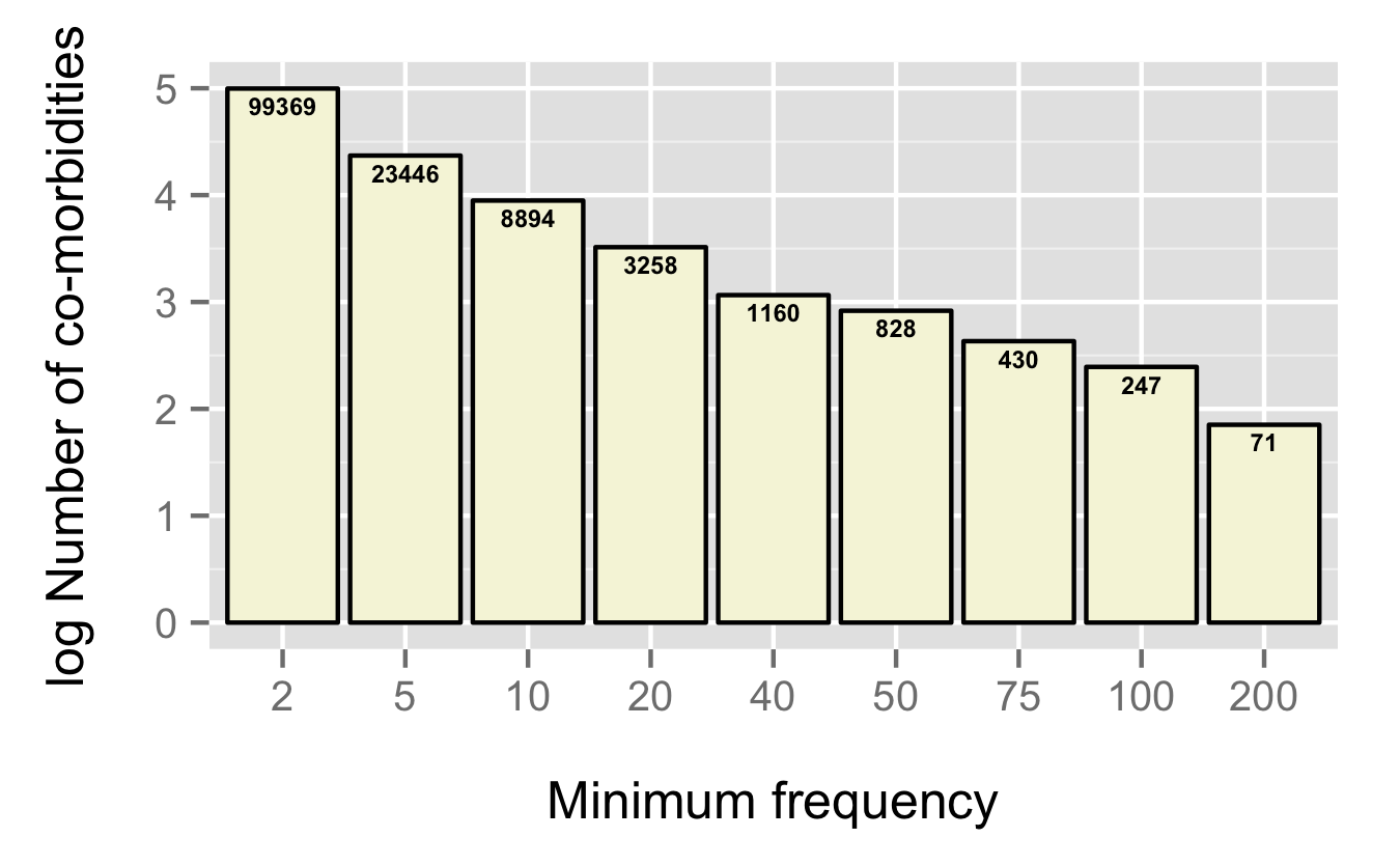
Having said that, we work with what we currently have – and it’s quite sparse. In fact the 28K case studies represent just 0.16% of all possible co-morbidities. Within the set of just under 600K unique observed co-morbidities, the bulk occur just once. For the rest of the analysis we ignore these singleton co-morbidities (leaving us with 513,997  co-morbidities). It’s interesting to see the distribution of frequencies of co-morbidities. The first figure plots the number of co-morbidities that occur at least N times – 99,369 co-morbidities occur 2 or more times in the dataset and so on.

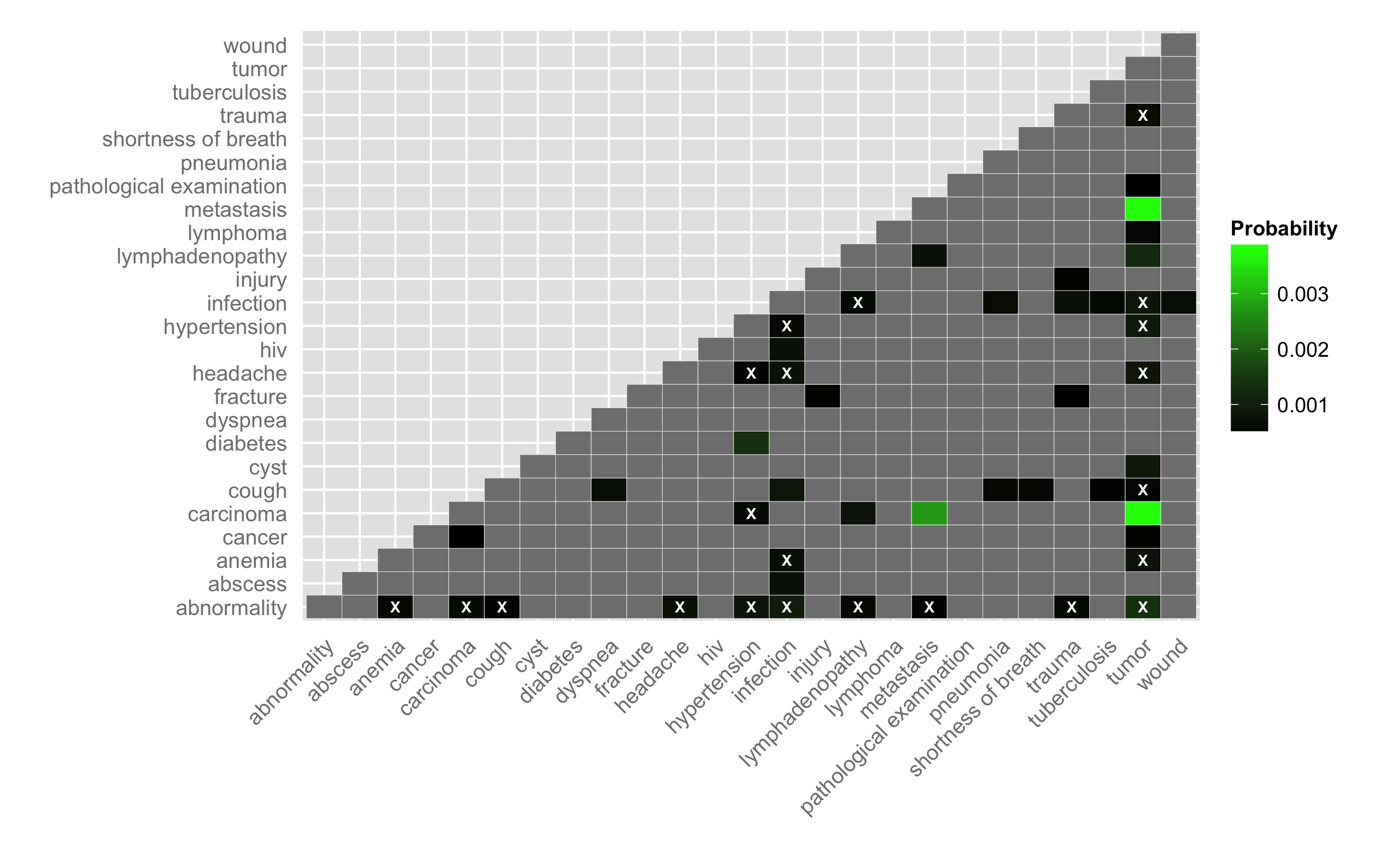
Another way to visualize the data is to plot a pairwise heatmap of conditions. For pairs of conditions that occur in the cases dataset we can calculate the probability of occurrence (i.e., number of times the pair occurs divided by the number of pairs). Furthermore, using a sampling procedure we can evaluate the number of times a given pair would be selected randomly from the pool of conditions. For the current analysis, I used 1e7 samples and evaluated the probability of a co-morbidity occurring by chance. If this probability is greater than the observed probability I label that co-morbidity as not different from random (i.e., insignificant). Ideally, I would evaluate a confidence interval or else evaluate the probability analytically (?).

For the figure below, I considered the 48 co-morbidities (corresponding to 25 unique conditions) that occurred 250 or more times in the dataset. I display the lower triangle for the heatmap – grey indicates no occurrences for a given co-morbidity and white X’s identify co-morbidities that have a non-zero probability of occurrence but are not different from random. As noted above, some of these pairs are not particularly informative – for example, tumor and metastasis occur with a relatively high probability, but this is not too surprising

Probability of occurrence for co-morbidities occurring more than 250 times

It’s pretty easy to modify co-morbidity.py to look at other sets of co-morbidities. Ideally, however, we would precompute probabilities for all co-morbidities and then support interactive visualization (maybe using D3).

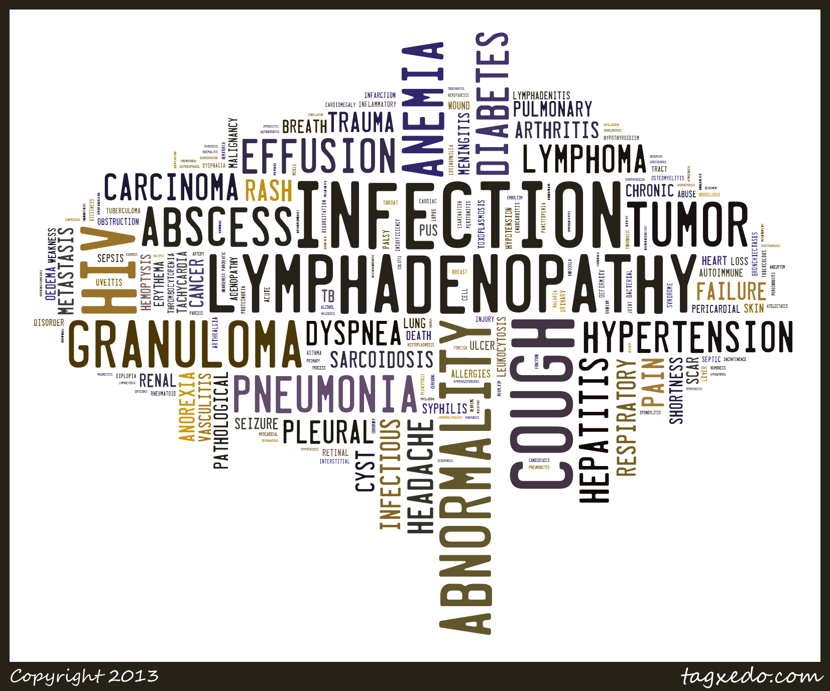
It’s also interesting to look at co-morbidities that include a specific condition. For example, lets consider tuberculosis (and all variants). There are 948 unique co-morbidities that include tuberculosis as one of the conditions. While the bulk of them occur just twice, there are a number with relatively large frequencies of occurrence – lymphadenopathy co-occurs with tuberculosis 203 times. Rather than tabulate the co-occurring conditions, we can use the frequencies to generate a word cloud, as shown below. As with the co-morbidity heatmaps, this could be easily automated to support interactive exploration. On a related note, it’d be quite interesting to compare the frequencies discussed here with data extracted from a live EHR system

A visualization of conditions most frequently co-occurring with tuberculosis

So far this has been descriptive – given the size of the data, we should be able to try out some predictive models. Future posts will look at the possibilities of modeling the case studies dataset.