For some time I have been thinking of the analogy between linguistics (and text mining of language data) and chemistry, specifically from the point of view of fragments (though, the relationship between the two fields is actually quite long and deep, since many techniques from IR have been employed in cheminformatics). For example, atoms and bonds can be considered an “alphabet” for chemical structures. Going one level up, one can consider fragments as words, which can be joined together to form larger structures (with the linguistic analog being sentences). In a talk I gave at the ACS sometime back I compared fragments with n-grams (though LINGO‘s are probably a more direct analog).

On these lines I have been playing with text mining and modeling tools in R, mainly via the excellent tm package. One of the techniques I have been playing around with is Latent Dirichlet Allocation. This is a generative modeling approach, allowing one to associate a document (composed of a set of words) with a “topic”. Here, a topic is a group of words that have a higher probability of being generated from that topic than another topic. The technique assumes that a document is comprised of a mixture of topics – as a result, one can assign a document to different topics with different probabilities. There have been a number of applications of LDA in bioinformatics with some applications focusing on topic models as way to cluster objects such as genes [1, 2], whereas others have used it in the more traditional document grouping context [3].

In text mining scenario, developing an LDA model for a set of documents is relatively straightforward (in R) – perform a series of pre-processing steps (mainly to standardize the text) such as converting everything to lower case, removing stopwords and so on. At the end of this one has a series of documents, each one being represented as a bag of words. The collection of words across all documents can be converted to a document-term matrix (documents in the rows, words in the columns) which is then used as input to the LDA routine.

Those familiar with building predictive models with keyed fingerprints will find this quite familiar – the individual bit positions represent structural fragments, thus are the chemical analogs of words. Based on this observation I wondered what I would get (and what it would mean) by applying a technique like LDA to a collection structures and their fragments.

My initial thought is that the use of LDA to determine a set of topics for a collection of chemical structures is essentially a clustering of the molecules, with the terms associated with the topics being representative substructures for that “cluster”. With these topics in hand, it wil be interesting to see what (or whether) properties (physical, chemical , biological) may be correlated with the clusters/topics identified. The rest of this post describes a quick first look at this, using ChEMBL as the source of structures and R for performing pre-processing and modeling.

Structures & fragments

We had previously fragmented ChEMBL (v8) in house, so obtaining the data was just a matter of running an SQL query to identify all fragments that occured in 50 or molecules and retrieving their structures and the molecules they were associated with. This gives us 190,252 molecules covered by 6,110 fragments. While a traditional text document-based modeling project would involved a series of pre-processing steps, the only one I need to perform in this scenario is the removal of small (and thus likely very common) fragments such as benzene – the cheminformatics equivalent of removing stopwords. (Ideally I would also remove fragments that already occur in other fragments – the cheminformatics equivalent of stemming)

The data file I have is of the form

where natom is the number of atoms in the fragment. The R code to generate (relatively) clean data, read to feed to the LDA function looks like:

In the code above, we rearrange the data to create “documents” – identified by a title (the molecule identifier) with the body of the document being the space concatenated SMILES for the fragments associated with that molecule. In other words, a molecule (document) is constructed from a set of fragments (words). With the data arranged in this form we can go ahead and reuse code from the tm and topicmodels packages.

Finally, we’re ready to develop some models, starting of with 6 topics.

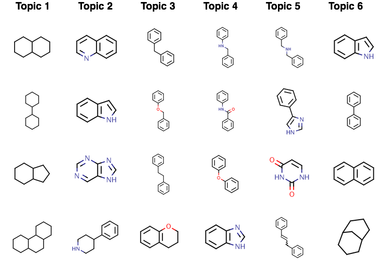
So, what are the topics that have been identified? As I noted above, each topic is really a set of “words” that have a higher probability of being generated by that topic. In the case of this model we obtain the following top 4 fragments associated with each topic (most likely fragments are at the top of the table):

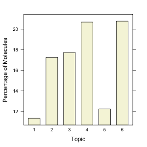
Visual inspection clearly suggests distinct differences in the topics – topic 1 appears to be characterized primarily by the lack of aromaticity, whereas topic 2 appears to be characterized by quinoline and indole type structures. This is just a rough inspection of the most likely “terms” for each topic. It’s also interesting to look at how the molecules (a.k.a., documents) are assigned to the topics. The barchart indicates the distribution of molecules amongst the 6 topics.

As with other unsupervised clustering methods, the choice of k (i.e., the number of topics) is tricky. A priori there is no reason to choose one over the other. Blei in his original paper used “perplexity” as a measure of the models generalizability (smaller values are better). In this case, we can vary k and evaluate the perplexity: with 6 topics the perplexity is 1122, with 12 topics it drops to 786 and with 100 topics it drops to 308 – you can see that it seems to continuously decrease with increase in number of topics (which has been observed elsewhere, though in my case, the hyperparameters are kept constant). Wallach et al have discussed various approaches to evaluating topic models.

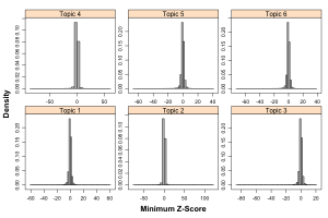
Numerical evaluation of these models is useful, but we’re more interested in how these assignments correlate with chemical or biological features. First, one could look at the structural homogenity of the molecules assigned to topics. For k = 6, this is probably not useful, as the individual groups are very large. With k = 100 one obtains a much more sensible estimate of homogeneity (but this is to be expected). Another way to evaluate the topics from chemical point of view is to look at some property or activity. Given that ChEMBL provides assay and target information for the molecules, we have many ways to perform this evaluation. As a brief example, we can consider activity distrbutions derived from the molecules associated with each topic. Most ChEMBL molecules have multiple activities associated with them as many are tested in multiple assays. To allow comparison we converted activities in a given assay to Z-scores, allow comparison of activitives across assays. Then for each molecule, we identified the minimum activity, only considering those activities that were annotated as IC₅₀ and as exact (i.e., not < or >). After removal of a few extreme outliers we obtain:

Clearly, within each group, the Z-scores cluster tightly around 0. It appears that the groups differentiate from each other in terms of the extreme values. Indeed plotting summary statistics for each group confirms this – in fact the median Z-score has a range of 0.05 and the mean Z-score a range of 0.11 across the six groups. In other words, the bulk of the groups are quite similar.

Other possibilities

The example shown here is rather simplistic and is the equivalent of unsupervised clustering. One obvious next step is to search the parameter space of the LDA model, evaluate different approaches to estimating the posterior distribution (EM or Gibbs sampling) and so on. A number of extensions to the basic LDA technique have been proposed, one of them being a supervised form of LDA.

It’d also be useful to look at this method on a slightly smaller, labeled dataset – I’ve run some preliminary experiments on the Bursi AMES but those results need a little more work. More generally, smaller datasets can be problematic as the number of unique fragments can be low. In addition fewer observations means that the estimates of the posterior distribution becomes fuzzier. One way around this is to develop a model on something like the ChEMBL dataset I used here and then apply that to smaller datasets. Obviously, this goes towards ideas of applicability – but given the size of ChEMBL, it may indeed “cover” many smaller datasets.

Is this useful?

At first sight, it’s an interesting method that identifies groupings in an unsupervised manner. Of course, one could easily run k-means or any of the hierarchical clustering methods to achieve the same result. However, the generative aspect of LDA models is what is of interest to me, but also seems the part that is difficult to map to a chemical setting – unlike topics in a document, which one can (usually) understand based on the likely terms for that topic, it’s not clear what a topic is for a collection of molecules in an unsupervised setting. And then, how does one infer the meaning of a topic from fragments? While it’s certainly true that certain fragments are associated with specific properties/activities, this is certainly not a given (unlike words, where each one does have an individual meaning). Furthermore, in an unsupervised setting like the one I’ve described here, fishing for a correlation between (some set of) properties and groupings of molecules is probably not the way to go.