Getting the GO into a Graph Data Structure

Today while working on a project I needed to get access to the Gene Ontology hierarchy. While there a number of GO browsers such as Amigo, I needed access to the raw data to generate a graph that I could then slice and dice. A few minutes with Python led to a simple solution.

The program parses the OBO 1.2 formatted GO data file (either by directly downloading it or from a local file) and outputs a flat dictionary listing the term ID’s, names, namespace etc and a network representation of the GO hierarchy in ncol format. It uses a simpleĀ  (and relatively non-robust) class to represent the data as an undirected graph (not really correct), though it’d be easy to use something like igraph to start doing some real network analysis. It’s certainly not a comprehensive solution, but I thought I’d put it out there.
Annotating Bioassays

I’ve been working for some time with the PubChem Bioassay collection – a set of 1293 assays that cover a range of techniques (enzymatic, phenotypic etc.), targets and sizes (from 20 molecules to 200,000 molecules). In addition, some assays are primary, high-throughput assays whereas a number of them are smaller, confirmatory assays. While an extremely valuable collection, one of the drawbacks is the lack of curation. This has led to some people saying that the data is too noisy to be useful. Yes, the noise is a problem, but I think there’s still useful data to extract and model.

One of the problems that I have faced is that while one can perform a full text search for assays on PubChem, there is no form of annotations on the assays themselves. One effect of this is that it is difficult to link an assay to other biological resources (though for enzymatic assays, one can determine a Pubmed protein identifier). While working on my bioassay network project, I needed annotations and I didn’t want to do it manually.

Continue reading

SALI Viewer Now on GitHub

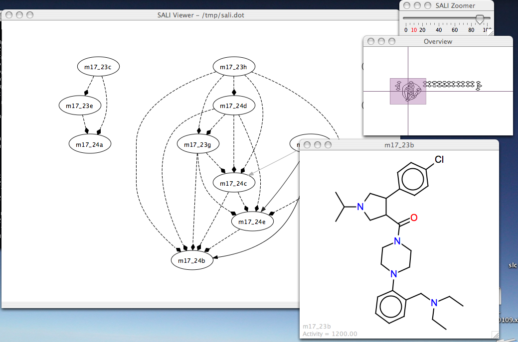
Last year, John Van Drie and I published two papers (here and here) on the Structure Activity Landscape Index, (SALI) which is a way to view SAR data as a network of compounds. Along with the paper ,I put up a simple Java application (licensed under the LGPL) to generate and explore these networks. – you only need to provide a file containing SMILES and activities. It’s based on ZGRViewer – a very slick GUI for Graphviz generated networks. I finally got around to reorganizing the code and putting it up on a GitHub repository. You can get more details of the application and the last stable version here.

sali-ss

ONS Solubility Predictions

Using the model deployment and prediction service, I put up the two linear regression models I had built so far (described in more detail here) While REST is nice, a simple web page that allows you to paste a set of SMILES and get back predictions is handy. So I whipped together a simple interface to the prediction service, allowing one to select a model, view the author-generated description and a get a nice (sortable!) table of predicted values. View it here. As noted in my previous post it’s not going to be very fast, but hopefully that will change in the future.

Deploying Predictive Models

Over the past few days I’ve been developing some predictive models in R, for the solubility data being generated as part of the ONS Solubility Challenge. As I develop the models I put up a brief summary of the results on the wiki. In the end however, we’d like to use these models to predict the solubility of untested compounds. While anybody can send me a SMILES string and get back a prediction, it’s more useful (and less work for me!) if a user can do it themselves. This requires that the models be deployed and made available as a web page or a service. Last year I developed a series of statistical web services based on R. The services were written in Java and are described in this paper. Since I’m working more with REST services these days, I wanted to see how easy it’d be to develop a model deployment system using Python, thus avoiding a multi-tiered system. With the help of rpy2, it turns out that this wasn’t very difficult.

Continue reading