While contributing to a book chapter on high content screening I came across the problem of characterizing screen quality. In a traditional assay development scenario the Z factor (or Z’) is used as one of the measures of assay performance (using the positive and negative control samples). The definition of Z’ is based on a 1-D readout, which is the case with most non-high content screens. But what happens when we have to deal with 10 or 20 readouts, which can commonly occur in a high content screen?

Assuming one has identified a small set of biologically relevant phenotypic parameters (from the tens or hundreds spit out by HCA software), it makes sense that one measure the assay performance in terms of the overall biology, rather than one specific aspect of the biology. In other words, a useful performance measure should be able to take into account multiple (preferably orthogonal) readouts. In fact, in many high content screening assays, the use of the traditional Z’ with a single readout leads to very low values suggesting a poor quality assay, when in fact, that is not the case if one were to consider the overall biology.

One approach that has been described in the literature is an extension of the Z’, termed the multivariate Z’. The approach was first described by Kummel et al, which develops an LDA model, trained on the positive and negative wells. Each well is described by N phenotypic parameters and the assumption is that one has pre-selected these parameters to be meaningful and relevant. The key to using the model for a Z’ calculation is to replace the N-dimensional values for a given well by the 1-dimensional linear projection of that well:

\(P_i = \sum_{j=1}^{D} w_j x_{ij} \)

where \(P_i\) is the 1-D projected value, \(w_j\) is the weight for the \(j\)’th pheontypic parameter and \(x_{ij}\) is the value of the \(j\)’th parameter for the \(i\)’th well.

The projected value is then used in the Z’ calculation as usual. Kummel et al showed that this approach leads to better (i.e., higher) Z’ values compared to the use of univariate Z’. Subsequently, Kozak & Csucs extended this approach and used a kernel method to project the N-dimensional well values in a non-linear manner. Unsurprisingly, they show a better Z’ than what would be obtained via a linear projection.

And this is where I have my beef with these methods. In fact, a number of beefs:

• These methods are model based and so can suffer from over-fitting. No checks were made and if over-fitting were to occur one would obtain a falsely optimistic Z’
• These methods assert success when they perform better than a univariate Z’ or when a non-linear projection does better than a linear projection. But neither comparison is a true indication that they have captured the assay performance in an absolute sense. In other words, what is the “ground truth” that one should be aiming for, when developing multivariate Z’ methods? Given that the upper bound of Z’ is 1.0, one can imagine developing methods that give you increasing Z’ values – but does a method that gives Z’ close to 1 really mean a better assay?  It seems that published efforts are measured relative to other implementations and not necessarily to an actual assay quality (however that is characterized).
• While the fundamental idea of separation of positive and negative control reponses as a measure of assay performance is good, methods that are based on learning this separation are at risk of generating overly optimistic assesments of performance.

A counter-example

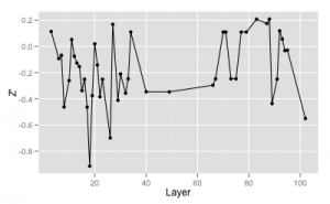
As an example, I looked at a recent high content siRNA screen we ran that had 104 parameters associated with it. The first figure shows the Z’ calculated using each layer individually (excluding layers with abnormally low Z’)

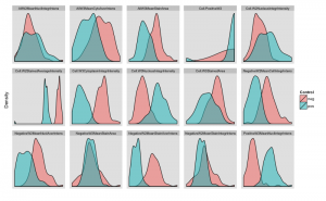
As you can see, the highest Z’ is about 0.2. After removing those with no variation and members of correlated pairs I ended up with a set of 15 phenotypic parameters. If we compare the per-parameter distributions of the positive and negative control responses, we see very poor separation in all layers but one, as shown in the density plots below (the scales are all independent)

I then used these 15 parameters to build an LDA model and obtain a multivariate Z’ as described by Kummel et al. Now, the multivariate Z’ turns out to be 0.68, suggesting a well performing assay. I also performed MDS on the 15 parameter set to get lower dimensional (3D, 4D, 5D, 6D etc) datasets and performed the same calculation, leading to similar Z’ values (0.41 – 0.58)

But in fact, from the biological point of view, the assay performance was quite poor due to poor performance of the positive control (we haven’t found a good one yet). In practice then, the model based multivariate Z’ (at least as described by Kummel et al can be misleading. One could argue that I had not chosen an appropriate set of phenotypic parameters – but I checkout a variety of other subsets (though not exhaustively) and I got similar Z’ values.

Alternatives

Of course, it’s easy to complain and while I haven’t worked out a rigorous alternative, the idea of describing the distance between multivariate distributions as a measure of assay performance (as opposed to learning the separation) allows us to attack the problem in a variety of ways. There is a nice discussion on StackExchange regarding this exact question. Some possibilities include

• Bhattacharya distance
• Mahalanobis distance
• Mantel test (though this is really a measure of correlation than a measure of effect size)
• The cross match test by Paul Rosenbaum (with a handy R package) – though this is more a measure of whether two distributions are different or not, rather than a distance between distributions
• An approach described by Loudin & Miettinen based on kernel density estimates and a 1-D Kolmogorov Smirnov test
  

It might be useful to perform a more comprehensive investigation of these methods as a way to measure assay performance